Examples
This page demonstrates how QCircuits can be used to simulate example quantum algorithms.
Producing Bell States
Example code producing each of the four entangled Bell states for a two-qubit system.
The circuit diagram is
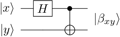
where |x⟩ and |y⟩ are each one of the computational basis states, |0⟩ or |1⟩.
E.g., \(|\beta_{00}⟩ = \frac{1}{\sqrt{2}} (|00⟩ + |11⟩)\).
Code:
import qcircuits as qc
from itertools import product


# Creates each of the four Bell states


def bell_state(x, y):
    H = qc.Hadamard()
    CNOT = qc.CNOT()

    phi = qc.bitstring(x, y)
    phi = H(phi, qubit_indices=[0])

    return CNOT(phi)


if __name__ == '__main__':

    for x, y in product([0, 1], repeat=2):

        print('\nInput: {} {}'.format(x, y))
        print('Bell state:')
        print(bell_state(x, y))
Quantum Teleportation
Code:
import qcircuits as qc
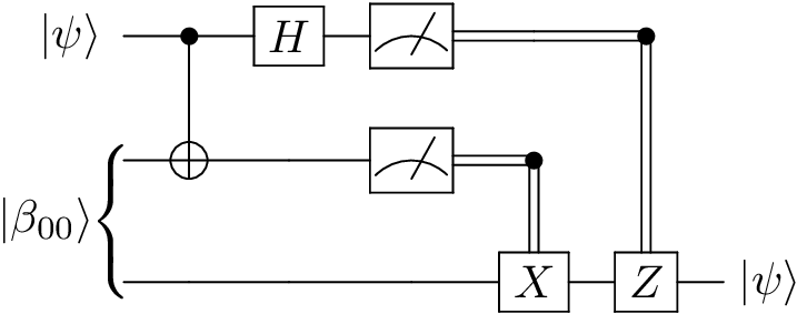
# Quantum Teleportation: transmitting two classical bits to transport a qubit state
# Alice has a qubit in a given quantum state.
# Alice and Bob have previously prepared a Bell state, and have since
# physically separated the qubits.
# Alice manipulates her hidden qubit and her half of the Bell state, and then
# measures both qubits.
# She sends the result (two classical bits) to Bob, who is able to reconstruct
# Alice's state by applying operators based on the measurement outcomes.
def quantum_teleportation(alice_state):
# Get operators we will need
CNOT = qc.CNOT()
H = qc.Hadamard()
X = qc.PauliX()
Z = qc.PauliZ()
# The prepared, shared Bell state
bell = qc.bell_state(0, 0)
# The whole state vector
state = alice_state * bell
# Apply CNOT and Hadamard gate
state = CNOT(state, qubit_indices=[0, 1])
state = H(state, qubit_indices=[0])
# Measure the first two bits
# The only uncollapsed part of the state vector is Bob's
M1, M2 = state.measure(qubit_indices=[0, 1], remove=True)
# Apply X and/or Z gates to third qubit depending on measurements
if M2:
state = X(state)
if M1:
state = Z(state)
return state
if __name__ == '__main__':
# Alice's original state to be teleported to Bob
alice = qc.qubit(theta=1.5, phi=0.5, global_phase=0.2)
# Bob's state after quantum teleportation
bob = quantum_teleportation(alice)
print('Original state:', alice)
print('\nTeleported state:', bob)
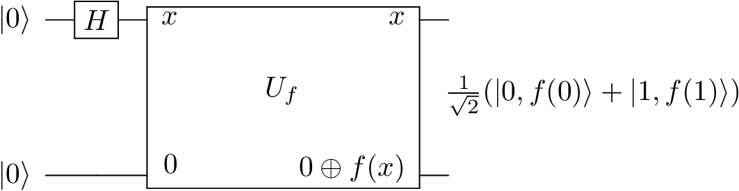
Quantum Parallelism
Code:
import qcircuits as qc
import numpy as np


# Example of quantum parallelism


# Construct a Boolean function
def construct_problem():
    answers = np.random.randint(0, 2, size=2)

    def f(bit):
        return answers[bit]

    return f


def quantum_parallelism(f):
    U_f = qc.U_f(f, d=2)
    H = qc.Hadamard()

    phi = qc.zeros(2)
    phi = H(phi, qubit_indices=[0])
    phi = U_f(phi)


if __name__ == '__main__':
    f = construct_problem()

    quantum_parallelism(f)
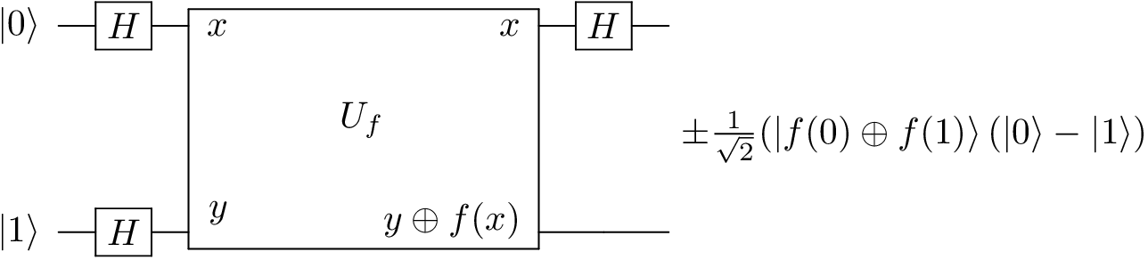
Deutsch’s Algorithm
Code:
import qcircuits as qc
import numpy as np


# Deutsch's Algorithhm:
# We use interference to determine if f(0) = f(1) using a single function evaluation.


# Construct a Boolean function that is constant or balanced
def construct_problem():
    answers = np.random.randint(0, 2, size=2)

    def f(bit):
        return answers[bit]

    return f


def deutsch_algorithm(f):
    U_f = qc.U_f(f, d=2)
    H = qc.Hadamard()

    phi = H(qc.zeros()) * H(qc.ones())
    phi = U_f(phi)
    phi = H(phi, qubit_indices=[0])

    measurement = phi.measure(qubit_indices=0)
    return measurement


if __name__ == '__main__':
    f = construct_problem()
    parity = f(0) == f(1)

    measurement = deutsch_algorithm(f)

    print('f(0): {}, f(1): {}'.format(f(0), f(1)))
    print('f(0) == f(1): {}'.format(parity))
    print('Measurement: {}'.format(measurement))
The Deutsch-Jozsa Algorithm
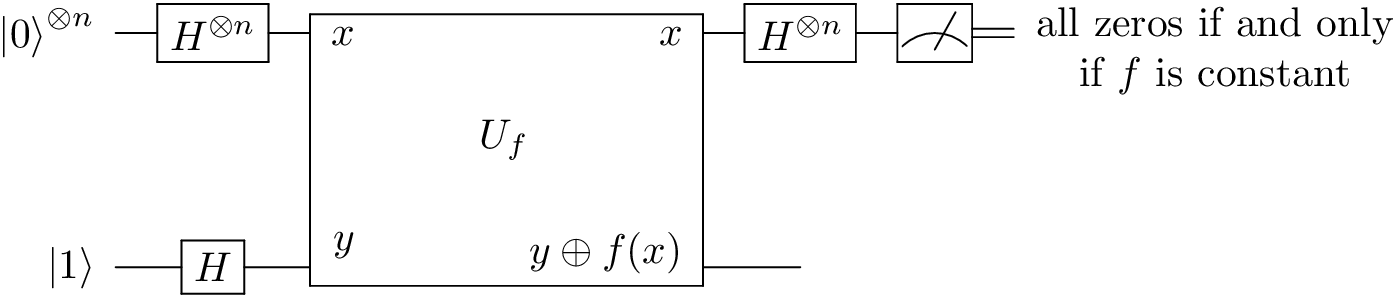
Code:
import qcircuits as qc
import numpy as np
import random


# Deutsch-Jozsa Algorithhm:
# We are presented with a Boolean function that is either constant or
# balanced (i.e., 0 for half of inputs, 1 for the other half).
# We make use of interference to determine whether the function is constant
# or balanced in a single function evaluation.


# Construct a Boolean function that is constant or balanced
def construct_problem(d=1, problem_type='constant'):
    num_inputs = 2**d
    answers = np.zeros(num_inputs, dtype=np.int32)

    if problem_type == 'constant':
        answers[:] = int(np.random.random() < 0.5)
    else: # function is balanced
        indices = np.random.choice(num_inputs, size=num_inputs//2, replace=False)
        answers[indices] = 1

    def f(*bits):
        index = sum(v * 2**i for i, v in enumerate(bits))

        return answers[index]

    return f


def deutsch_jozsa_algorithm(d, f):
    # The operators we will need
    U_f = qc.U_f(f, d=d+1)
    H_d = qc.Hadamard(d)
    H = qc.Hadamard()

    state = qc.zeros(d) * qc.ones(1)
    state = (H_d * H)(state)
    state = U_f(state)
    state = H_d(state, qubit_indices=range(d))

    measurements = state.measure(qubit_indices=range(d))
    return measurements


if __name__ == '__main__':
    d = 10
    problem_type = random.choice(['constant', 'balanced'])

    f = construct_problem(d, problem_type)
    measurements = deutsch_jozsa_algorithm(d, f)

    print('Problem type: {}'.format(problem_type))
    print('Measurement: {}'.format(measurements))
    print('Observed all zeros: {}'.format(not any(measurements)))
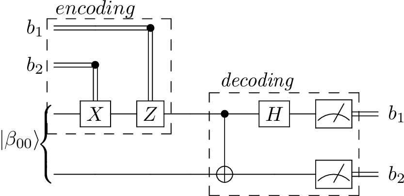
Superdense Coding
Code:
import qcircuits as qc
import numpy as np


# Superdense Coding: transmitting a qubit to transport two classical bits
# Alice and Bob have previously prepared a Bell state, and have since
# physically separated the qubits.
# Alice has two classical bits she wants to transmit to Bob.
# She manipulates her half of the Bell state depending on the values of those bits,
# then transmits her qubit to Bob, who then measures the system.


def superdense_coding(bit_1, bit_2):
    # Get operators we will need
    CNOT = qc.CNOT()
    H = qc.Hadamard()
    X = qc.PauliX()
    Z = qc.PauliZ()

    # The prepared, shared Bell state
    # Initially, half is in Alice's possession, and half in Bob's
    phi = qc.bell_state(0, 0)

    # Alice manipulates her qubit
    if bit_2:
        phi = X(phi, qubit_indices=[0])
    if bit_1:
        phi = Z(phi, qubit_indices=[0])

    # Bob decodes the two bits
    phi = CNOT(phi)
    phi = H(phi, qubit_indices=[0])
    measurements = phi.measure()
    return measurements


if __name__ == '__main__':
    # Alice's classical bits she wants to transmit
    bit_1, bit_2 = np.random.randint(0, 2, size=2)

    # Bob's measurements
    measurements = superdense_coding(bit_1, bit_2)

    print("Alice's initial bits:\t{}, {}".format(bit_1, bit_2))
    print("Bob's measurements:\t{}, {}".format(measurements[0], measurements[1]))
Phase Estimation
We are give a black-box d-qubit operator U and one of its eigenstates. The task is to estimate the phase of the corresponding eigenvalue, storing the result in a t-qubit register.
Code:
import qcircuits as qc
import numpy as np
from scipy.stats import unitary_group


# Phase estimation
# We are given a black-box unitary operator, and one of its eigenstates.
# The task is to estimate the phase of the corresponding eigenvalue.
# This is done making use of the efficient inverse quantum Fourier transform.


# Prepares a state that when the inverse Fourier transform is applied,
# unpacks the binary fractional expansion of the phase into the
# first t-qubit register.
def stage_1(state, U, t, d):
    state = qc.Hadamard(d=t)(state, qubit_indices=range(t))

    # For each qubit in reverse order, apply the Hadamard gate,
    # then apply U^(2^i) to the d-qubit register
    # conditional on the state of the t-i qubit in the
    # t-qubit register.
    for idx, t_i in enumerate(range(t-1, -1, -1)):
        U_2_idx = U
        for app_i in range(idx):
            U_2_idx = U_2_idx(U_2_idx)
        C_U = qc.ControlledU(U_2_idx)
        state = C_U(
            state,
            qubit_indices=[t_i] + list(range(t, t+d, 1))
        )

    return state


# The t-qubit quantum Fourier transform
def QFT(t):
    Op = qc.Identity(t)
    H = qc.Hadamard()

    # The R_k gate applies a 2pi/2^k phase is the qubit is set
    C_Rs = {}
    for k in range(2, t+1, 1):
        R_k = np.exp(np.pi * 1j / 2**k) * qc.RotationZ(2*np.pi / 2**k)
        C_Rs[k] = qc.ControlledU(R_k)

    # For each qubit in order, apply the Hadamard gate, and then
    # apply the R_2, R_3, ... conditional on the remainder of the qubits
    for t_i in range(t):
        Op = H(Op, qubit_indices=[t_i])
        for k in range(2, t+1 - t_i, 1):
            Op = C_Rs[k](Op, qubit_indices=[t_i + k - 1, t_i])

    # We have the QFT, but with the qubits in reverse order
    # Swap them back
    Swap = qc.Swap()
    for i, j in zip(range(t), range(t-1, -1, -1)):
        if i >= j:
            break
        Op = Swap(Op, qubit_indices=[i, j])

    return Op


# The t-qubit inverse quantum Fourier transform
def inv_QFT(t):
    return QFT(t).adj


# Do phase estimation for a random d-qubit operator,
# recording the result in a t-qubit register.
def phase_estimation(d=2, t=8):
    # a d-qubit gate
    U = unitary_group.rvs(2**d)
    eigvals, eigvecs = np.linalg.eig(U)
    U = qc.Operator.from_matrix(U)

    # an eigenvector u and the phase of its eigenvalue, phi
    phi = np.real(np.log(eigvals[0]) / (2j*np.pi))
    if phi < 0:
        phi += 1
    u = eigvecs[:, 0]
    u = qc.State.from_column_vector(u)

    # add the t-qubit register
    state = qc.zeros(t) * u

    state = stage_1(state, U, t, d)
    state = inv_QFT(t)(state, qubit_indices=range(t))
    measurement = state.measure(qubit_indices=range(t))
    phi_estimate = sum(measurement[i] * 2**(-i-1) for i in range(t))

    return phi, phi_estimate


if __name__ == '__main__':
    phi, phi_estimate = phase_estimation(d=2, t=8)

    print('True phase: {}'.format(phi))
    print('Estimated phase: {}'.format(phi_estimate))
Grover’s Algorithm
We are given a black-box boolean function f(x) that evaluates to 1 for exactly one value of x. Grover’s algorithm finds the solution with resources proportional to the square root of the size of the search space.
Code:
import qcircuits as qc
import numpy as np
import random


# Grover's algorithm (search)
# Given a boolean function f, Grover's algorithm finds an x such that
# f(x) = 1.
# If there are N values of x, and M possible solutions, it requires
# O(sqrt(N/M)) time.
# Here, we construct a search problem with 1 solution amongst 1024
# possible answers, and find the solution with 25 applications of
# the Grover iteration operator.


# Construct a Boolean function that is 1 in exactly one place
def construct_problem(d=10):
    num_inputs = 2**d
    answers = np.zeros(num_inputs, dtype=np.int32)
    answers[np.random.randint(0, num_inputs)] = 1

    def f(*bits):
        index = sum(v * 2**i for i, v in enumerate(bits))

        return answers[index]

    return f


def grover_algorithm(d, f):
    # The operators we will need
    Oracle = qc.U_f(f, d=d+1)
    H_d = qc.Hadamard(d)
    H = qc.Hadamard()
    N = 2**d
    zero_projector = np.zeros((N, N))
    zero_projector[0, 0] = 1
    Inversion = H_d((2 * qc.Operator.from_matrix(zero_projector) - qc.Identity(d))(H_d))
    Grover = Inversion(Oracle, qubit_indices=range(d))

    # Initial state
    state = qc.zeros(d) * qc.ones(1)
    state = (H_d * H)(state)

    # Number of Grover iterations
    angle_to_rotate = np.arccos(np.sqrt(1 / N))
    rotation_angle = 2 * np.arcsin(np.sqrt(1 / N))
    iterations = int(round(angle_to_rotate / rotation_angle))
    for i in range(iterations):
        state = Grover(state)

    measurements = state.measure(qubit_indices=range(d))
    return measurements


if __name__ == '__main__':
    d = 10

    f = construct_problem(d)
    bits = grover_algorithm(d, f)

    print('Measurement: {}'.format(bits))
    print('Evaluate f at measurement: {}'.format(f(*bits)))